A perfect curve shape of analytical 2D
data objects include a constant base level value, where no signals
are observed. This base level is called the baseline of a 2D data object.
Because of changes in experimental conditions during measurement, temperature
influences or any other interference, the baseline sometimes drifts away
from its original base level. In this case, the baseline of a 2D data
object might be corrected after a measurement has been completed using
the baseline correction
function of the software. It might be applied, whenever consecutive operations
are required like ATR correction or finding peaks.
Several baseline algorithms are available as described in the following:
Polyline algorithm
Horizontal algorithm
Peak detection algorithm
Linear least squares regression algorithm
Two point algorithm
Spline algorithm
AirPLS algorithm
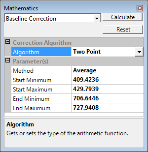
To select one of the algorithms, choose
the entry from the algorithm drop down
box in the Mathematics tab.
Each algorithm provides a set of individual parameters, which can be adjusted
after selection.
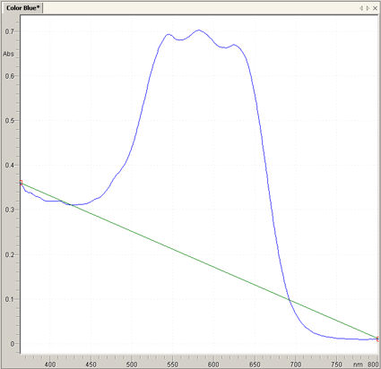
This algorithm shows a linear baseline drawn directly between first
and last data point of the current visible part of the 2D data object
in the data view. The end points of the line possess baseline knots (red
squares) which can be moved to adjust bias and slope of the line:
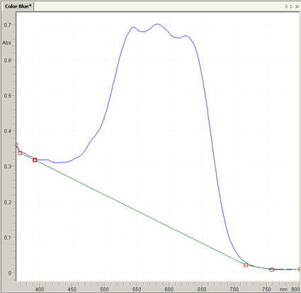
Additional knots
can be added optionally to get a polygonal line for correction. Please review the Baseline
Correction section in the chapter "Commands" to learn how to
add and remove baseline knots. After adding some baseline knots,
correction can be carried out.
The polyline algorithm offers an additional autodetect
option. Choosing this option will modify the polyline so that the baseline
knots of the resulting corrected spectra will lie on the x-axis:
Autodetect selected: All spectra will be corrected so
that the selected baseline knots will lie on the x-axis with an y-value
of 0.
Autodetect unselected: The selected polyline will used
"as is" to correct the spectra. The resulting baseline may not
coincide exactly with the x-axis.
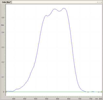
The corrected data object looks like this:
After correction a new baseline will be proposed automatically for subsequent
correction.
Which region is considered for baseline correction?
Baseline correction is only performed on the area covered by the line!
Data points outside the area remain unchanged.
The baseline will be corrected by using a horizontal line. In principle
this algorithm works like an offset correction. The entered value will
be subtracted from the entire spectrum, thus shifting it up or down for
a certain amount. Therefore this algorithm is especially useful for correcting
spectra with a constant offset. The correction value can either be entered
by moving the horizontal line directly in the spectrum or by entering
a numerical value into the parameter "absolute height". By clicking
the Reset
button the horizontal line and the parameter "absolute height"
will automatically be set to the minimum intensity present in the spectrum.
You can use this algorithm to correct positive or negative offsets.
A polygonal fit function will be determined automatically, which follows
the slope of the graph of the 2D data object by neglecting detected peaks.
Significant changes in the bias indicate the starting and ending point
of a peak signal. These regions will be excluded from baseline detection
automatically. The user might assist the automatic peak detection algorithm
by adjusting the following parameters:
This parameter indicates, whether adjacent or overlapping peaks will
be interpreted as a single peak or multiple peaks. If the flag is set
true, such overlapping peaks will be ignored and identified as one peak.
The baseline of the following spectrum excerpt is shown in the figure
below (red line):
If the parameter is set false, at least one data point between the end
of the first peak and the starting point of the next peak will be interpreted
as a base line point. In this case, the same baseline correction detects
multiple peaks within the displayed area from above. The baseline follows
the red line in this case:
This parameter controls the peak detection concerning the minimum peak
height. It is a threshold value relative from the imaginary base line
along the graph slope, that must be overridden to identify a peak. The
minimum relative peak height is given in fractions of y-axis units.
This parameter controls the peak detection concerning the minimum peak
width. A minimum expected peak width is adjusted here. This value might
alter depending on the data type. The minimum estimated peak width is
given in fractions of x-axis units.
This baseline correction algorithm facilitates the Standard
Normal Variate correction. Besides the noise and background correction
the overall graph slope can be detrended. A polynomial fit function is
applied for detrending.
Detrend
Detrending can be included into the baseline correction or not. The
following parameter settings are available:
None
No detrending is performed.
Polynomial Fit
A polynomial fit function is applied for detrending.
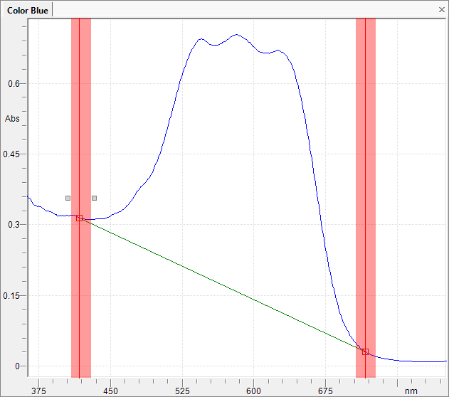
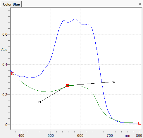
The baseline will be corrected by a line defined by two points. These
endpoints can be automatically calculated from a predefined region in
the spectrum. This is useful for sets of spectra which exhibit slight
shifts. Several methods calculating the start and end point are available.
The selection for the two point baseline correction looks like this:
The endpoint preselection is done by moving the red selection rectangles
to the desired position. The width of the selection rectangle can be adjusted
by the grey tracker boxes and defines the region of points from which
the actual endpoint will be calculated by one of the following methods.
The actual calculated endpoints are shown as red vertical lines with red
boxes inside the selection rectangles.
Single
Two distinct points are directly selected as endpoints. The point are
show as red vertical lines without selection areas in the spectrum. This
is similar to the simple line algorithm.
Average
The endpoints are calculated as the average
of the group of points that are defined by the selection rectangle.
Minimum
The endpoints are calculated as the minimum
of the group of points that are defined by the selection rectangle.
Maximum
The endpoints are calculated as the maximum
of the group of points that are defined by the selection rectangle.
None
No endpoint selection algorithm is used.
Alternatively the numerical values can be entered directly using the
parameter sets Startx, EndX or Start Minimum, Start Maximum, End Minimum
and End Maximum:
The two-point algorithm is also part of the baseline correction used
in the command thickness correction. Please refer to the chapter thickness
correction for a detailed description of the selection methods.
The spline algorithm works similar to the Polyline algorithm except
for the handling of the baseline knots. When using the spline algorithm,
each baseline knot will have additional spline controls to help adjusting
the line shape. By moving the spline controls the user is able to accurately
adapt the baseline shape to the spectrum. The following picture shows
an example of an intermediate baseline knot with two spline controls:
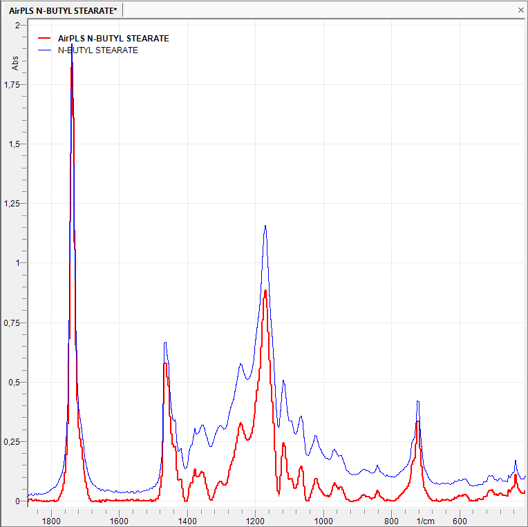
The AirPLS algorithm is a baseline correction algorithm which works completely on its own and that does not require any user intervention or prior information, such as peak detection etc.
Parameters provided by user are only the maximum amount of iteration and a Lambda.
Iterations
The maximum amount of iterations the algorithm should do.
Lambda
A detail parameter for the algorithm.
Which Lambda fits my needs?
The lower Lambda is set, the more detailed the algorithm will work but will also need more time. Little shifts in baseline will be more likely corrected with a low Lambda. In most cases the default Parameter (Lambda = 10) is sufficient for baseline correction.